How the Kalman Filter's Predict-Update Cycle Minimizes Error in Time-Series State Estimation

An autonomous navigation computer does not actually know where its vehicle is; it only knows where its mathematical model predicted it would be, and what its noisy sensors currently report. At every time step, the system must decide how much to trust its own internal physics model versus the external data arriving from the real world. This continuous arbitration is governed by the Kalman filter, a recursive algorithm that minimizes error by calculating the optimal mathematical middle ground between a flawed prediction and a flawed measurement.[6][7]

MathWorks documentation notes that "the filter's algorithm is a two-step process: the first step predicts the state of the system, and the second step uses noisy measurements to refine the estimate of system state." In the prediction phase, the filter uses a state transition model—the known physical laws governing the system, such as velocity and acceleration—to project the current state forward in time. Because physical models cannot account for every external variable, this prediction introduces process noise, meaning the uncertainty of the estimate strictly increases during this phase.[7][8]

The update phase introduces the empirical data. The system takes a reading from its sensors, which inherently contain measurement noise due to hardware limitations or environmental interference. The filter then calculates the Kalman Gain, a dynamic weighting factor that determines whether the prediction or the measurement is mathematically more reliable. "The Kalman Filter is an algorithm for estimating and predicting the state of a system in the presence of uncertainty, such as measurement noise or influences of unknown external factors," according to KalmanFilter.net.[8][9]

If the sensor data has a high variance, indicating high uncertainty, the Kalman Gain shifts the weight toward the internal prediction. Conversely, if the physical model has drifted and accumulated high uncertainty, the gain shifts the weight toward the new sensor measurement. By multiplying the difference between the prediction and the measurement by this optimal gain, the filter computes a posterior state estimate. The state estimate is often represented as a multi-dimensional vector—for example, a 4-by-1 column vector tracking position and velocity in two dimensions, paired with a 4-by-4 covariance matrix tracking the uncertainty.[6][9]

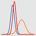
The mathematical power of this cycle lies in its effect on the system's overall uncertainty. Because the filter fuses two independent sources of information, the variance of the updated estimate is mathematically guaranteed to be lower than the variance of either the prediction or the measurement alone. In a standard 1-dimensional application, the updated variance is calculated as the inverse of the sum of the inverses of the prior and measurement variances. The uncertainty matrix shrinks, and the system becomes more confident in its estimated state.[6][8]

This variance-minimization property was first published by Rudolf E. Kálmán in a seminal 35-page paper in 1960 in the Journal of Basic Engineering. Originally developed for aerospace applications, the algorithm provided a computationally efficient way to estimate the internal state of linear dynamic systems using only the present input measurements and the previously calculated state, requiring no historical data storage.[1][6]

Today, the algorithm extends far beyond linear aerospace trajectories. In meteorology, reduced-order Kalman filters are deployed to estimate atmospheric states, fusing satellite observations with massive fluid-dynamics models to forecast weather patterns, as detailed in a 2001 study by the American Meteorological Society. In industrial robotics, robust estimation theory is combined with Kalman filtering to fuse multi-source information in highly non-linear systems, allowing autonomous machines to navigate unpredictable factory floors.[2][3]

Despite its ubiquity, the standard Kalman filter is strictly optimal only under specific mathematical conditions. The system must be linear, and both the process noise and the measurement noise must follow a perfect Gaussian distribution. When these conditions are violated, engineers must deploy variants like the Extended Kalman Filter, which linearizes non-linear models via differential equations, or the Unscented Kalman Filter, which uses deterministic sampling to approximate the probability distribution.[5][6]

The filter's reliance on accurate noise covariance matrices remains its primary vulnerability. If an engineer poorly estimates the inherent noise of a sensor—for instance, failing to calculate that a thermometer fluctuating by an average of 0.8 degrees produces a variance of 0.64—the Kalman Gain will assign incorrect weights. This causes the filter to trust flawed data and diverge from the true state. The algorithm can only minimize error if the bounds of that error are accurately defined.[4][8]

By continuously cycling between predicting the future and correcting those predictions with empirical reality, the algorithm ensures that the inevitable errors of both mathematics and hardware are mathematically constrained. The system finalizes its posterior estimate, updates its covariance matrix, and immediately feeds those values back into the model to begin the next prediction cycle.[6][8]