The Mechanics of Nodal Pricing: How Locational Marginal Pricing (LMP) Resolves Grid Congestion

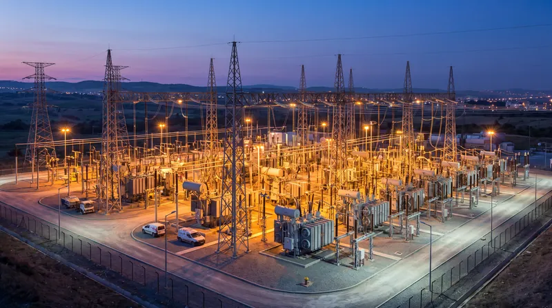
Electricity is not priced uniformly. In restructured wholesale markets across the United States—including PJM, ERCOT, CAISO, and ISO New England—grid operators calculate the cost of power at thousands of distinct physical locations, known as nodes. This granular system, called Locational Marginal Pricing (LMP), ensures that the wholesale price of electricity accurately reflects the physical realities of generating and delivering it across a complex network.[1][2]

The core problem LMP solves is that electricity must be consumed the exact moment it is generated, and the transmission lines connecting supply to demand have strict physical limits. When a transmission line reaches its maximum thermal or stability capacity, the grid operator cannot simply send more power down that wire, even if a cheap wind farm or natural gas plant is ready to produce it.

To manage this delicate balance, the LMP algorithm runs continuously, solving a massive optimization problem every five minutes. It takes generation bids from power plants and demand forecasts from utilities, then dispatches the lowest-cost combination of generators that can meet the load without overloading any transmission lines. The resulting clearing price at each specific node is the LMP.[1]

The LMP is not a single arbitrary number; it is the mathematical sum of three distinct components: the marginal cost of energy, the marginal cost of congestion, and the marginal cost of losses. By isolating these factors, the market provides total transparency into exactly what is driving the cost of power at any given moment.[2]

The energy component serves as the baseline. It represents the cost to serve the next increment of demand on the system if there were absolutely no transmission constraints and no power lost as heat along the wires. In a perfectly unconstrained grid, this energy component would be the only factor, and the price of electricity would be identical everywhere, set by the single most expensive generator needed to meet total system demand.[2]

The congestion component is where the market reflects physical reality. When a transmission line is fully loaded, the grid operator must dispatch a more expensive generator located closer to the demand to avoid overloading the line. The congestion component is the price difference between the cheap power that cannot be delivered and the expensive power that must be used instead.

This congestion pricing acts as both a penalty and an incentive. For generators trapped behind a bottleneck—such as wind farms in West Texas or the Dakotas—the congestion component becomes negative, driving their local LMP down and signaling them to reduce output. For generators on the demand side of the bottleneck, the congestion component is positive, driving their local LMP up and compensating them for running when cheaper remote power cannot reach the load.[3]

The final piece of the equation is the loss component. As electricity travels over long distances, a small percentage of it dissipates as heat due to the inherent electrical resistance of the transmission wires. The loss component accounts for the cost of generating the extra power needed to make up for this physical dissipation. Nodes located further from generation centers typically see slightly higher loss components.[2]

Together, these three components create a highly dynamic and granular price map. During normal operations, LMPs across a region might hover within a few dollars of each other. But during extreme weather, sudden power plant failures, or unexpected demand surges, congestion can cause prices at neighboring nodes to diverge by hundreds or even thousands of dollars per megawatt-hour.[3]

This volatility is entirely intentional. The sharp price separation created by nodal pricing provides the financial justification for long-term grid upgrades. When developers see persistent, high congestion costs at a specific node, it signals exactly where a new transmission line, a grid-scale battery, or a flexible demand resource will be most profitable and most beneficial to the system.

However, this granularity also introduces significant basis risk for market participants. A utility or industrial consumer that buys power at a regional hub price but consumes it at a specific constrained node can face massive financial exposure if congestion drives their local LMP significantly higher than the hub price they contracted for.[3]

To manage this risk, grid operators offer Financial Transmission Rights (FTRs) or Congestion Revenue Rights (CRRs). These financial instruments allow market participants to hedge against the volatility of the congestion component, essentially locking in the price difference between two nodes ahead of time and providing budget certainty in an otherwise fluctuating market.[1][3]

As the grid transitions to a higher penetration of renewable energy, the mechanics of LMP are becoming even more critical. Wind and solar resources are often located far from population centers, increasing the frequency and severity of transmission congestion. Nodal pricing ensures that the market accurately values the flexibility needed to balance these intermittent resources and incentivizes building generation where the grid can actually accommodate it.[3]

Ultimately, Locational Marginal Pricing functions as the financial nervous system of the modern power grid. By translating the physical laws of electricity into economic signals, it forces the market to respect the limits of the transmission network while continuously driving private investment toward the most constrained and valuable areas of the infrastructure.[3]